Whose the best table tennis player in the office?

Recently, our office acquired a table tennis table. After several weeks of impromptu matches between a variety of office folk, the inevitable question arose - whose the best player in the office?

Being a data scientist, I sort to answer this question using data…and science.

The very first activity, record the data! So we set up a message board to record the outcomes of all matches. All match outcomes could now be recorded consistently in a centralised place.

Secondly, we needed a way to use this data to rank our participants. Since matches are impromptu, not all players may have the chance to play all other players. Due to different work schedules, naturally some players play more often than others. Also, we needed a system to account for the strength of the opposition that is played. What we needed was a class of models that estimate skill / ability based on data of who has played who.

These models are very common in sports and gaming. Several models exist to do this, none more famous than the familiar ELO system, used in chess. I’ve used a variant of an ELO model in my own AFL modeling in the past. However, for our table tennis comp, rather then apply a simple ELO model, I decided to take it up a notch and deploy a Bayesian probabilistic model.

Thinking about ratings probabilistically (warning: math!)

The idea of rating players on a scale means assigining them numerical ability scores (\(\alpha\)) that somehow map to how good or bad they are. Rank is determined through ordering the players by their inferred ability.

In a probabalistic framework, this means we need to come up with a probability distribution that describes how the match outcome is related to player a and b’s numerical ability (\(\alpha_a\) and \(\alpha_b\)). That is, we need to find:

\[ P(M|\alpha_a, \alpha_b, \beta) \]

which literally means “the probability of observing match outcome \(M\) given parameters \(\alpha_a\), \(\alpha_b\), and \(\beta\) as determined by the assumed probability mass function \(P\)”. Here \(\beta\) are parameters other than the numerical ratings that describe the probability mass function.

As an example, this could be a normal distribution with a mean (\(\mu\)) equal to the difference in ratings and a variance parameter \(\sigma\) i.e.,

\[ P(M|\alpha_a, \alpha_b, \beta) = N(M|\mu = \alpha_a - \alpha_b, \sigma = \beta) = \frac{1}{{\sigma \sqrt {2\pi } }}e^{{{ - \left( {x - \mu } \right)^2 / 2\sigma^2}}} \] But, it doesn’t have to be a normal distribution and the choice of distribution really depends on the sport’s scoring mechanism. Formally, this probability distribution is known as the “likelihood”. If we knew each player’s numerical ability and the other parameters \(\beta\), we could find the chance (probability or “likelihood”) of the data that was observed by sticking the values through the likelihood function.

The other thing we need is data. Once we have data on match outcomes, we can find (“learn” or “calculate”) the ability scores for each player (and also other parameters that we might need, i.e., \(\beta\) ) using some kind of optimisation routine maximising the following function:

\[ \sum_i log[P(M_i|\alpha_a, \alpha_b, \beta)] \] where \(i\) denotes the \(i^{th}\) data point (in this case game).

This is called the “log-likelihood” function. By finding the parameters that maximise this function, we are finding player scores that yield the highest chance of the data that we observed to be generated under the assumed likelihood function. That’s a mouthful, but it essential means we are maximising the probability of the data being generated.

Thinking about scoring and rating probabilistically has it’s advantages. For one thing, we are explicitly considering the data generating process which is important when we want to extend the concept to sports that have different types of scoring mechanisms. For example, in a high scoring sport like Australian Football, it is common to use a normal distribution to approximate the likelihood function of the margin. This is because scoring is quite high and margins have quite a large spread. Assuming a continuous margin is mostly adequate. However, in a sport like soccer, where goals are basically discrete integers, it is very common to use discrete distributions (e.g., a Skellam), because you cannot reasonably assume continuous goal differences.

The likelihood function for table tennis

We can’t use a normal distribution for table tennis. The margin in table tennis is always an integer and can’t be less than 2. In fact, the mechanics of scoring in table tennis are completely different to AFL or Soccer. In AFL or Soccer, it’s about kicking the most goals in fixed period of time. But table tennis (and tennis for that matter) matches continue to infinity until a winning condition is met. Who could forget the famous Isner–Mahut match at the 2010 Wimbledon Championships?

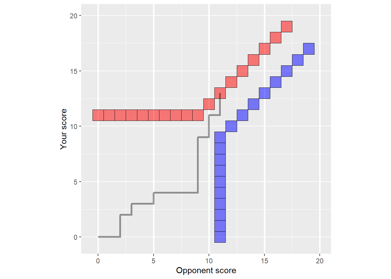
In our office comp, we play first person to reach 11 with margin >=2. If 11 is reached with a margin <2, then overtime is played until a player wins two points in a row. A nice diagram of how a table tennis match might progress is shown here (which I copied from here). When the score worm (grey) hits either the red or the blue boundaries, the match will finish.

When this dawned on me, I realised that we needed to create a completely new likelihood function in order to adequately describe the data generating process. So I set about deriving, by hand, a new likelihood function for table tennis. Eventually after about 3 hrs of thinking about it, this is what I came up with:

\[ P(y|p, X_{wins}) = \begin{cases} \frac{1}{W}{10+y \choose 10}p^{11}(1-p)^y & y<10\\ \frac{1}{W}{10+10 \choose 10}p^{10}(1-p)^{10}(2p(1-p))^{y-10}p^2 & y\ge10\\ \end{cases} \]

where

\[ W = \sum_{y=0}^9 {10+y \choose 10}p^{11}(1-p)^y + {10+10 \choose 10}\frac{p^{12}(1-p)^{10}}{1-2p(1-p)} \]

which describes the probability mass of the losing player scoring \(y\) points at the end of the match if the probability of the winning player winning each individual point is \(p\) (recall that if the losing player scores \(y\) points, the winner has necessarily scored \(\text{max}(11,y+2)\) points).

If this looks crazy complicated to you, you’re right, it is. It isn’t a nice formula like a normal distribution or even a Skellam. But it is a better model for table tennis because it better simulates the actual data generating process, which in statistical modelling is one of the most important things to get right. I’ve put a much more detailed derivation in the appendix of this blog if anyone wants to go through it.

Note that while I definitely derived this independently, I also found this paper, which basically derives the same thing (and a whole lot more), but 10 years earlier. It’s heartening to know that I still have maths skills and what I derived was correct. But it’s also a good lesson that it pays dividends to look before you try something yourself, because chances are someone has already had a crack.

What does this likelihood function look like?

To get a better feel for how this likelihood behaves, take a look at the heat map below. This shows the variation in the probability mass with both losing score, \(y\) and probability to win a game, \(p\).

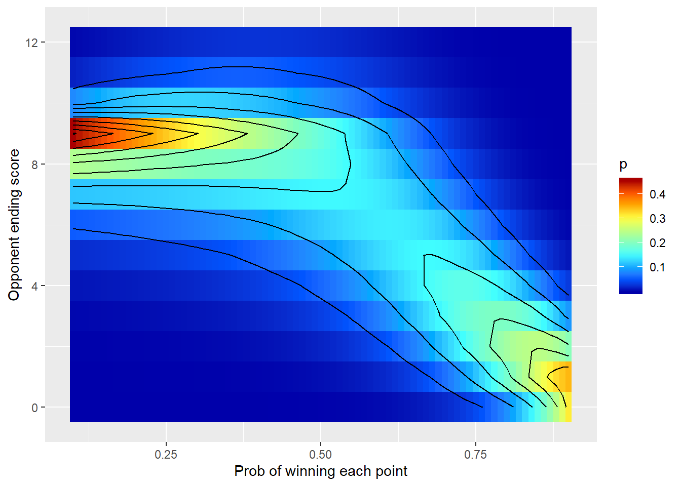
This graph tells us three things:

1. If the winner had a lower probability of winning each point (\(p\)), then its much more likely that the game will finished with the loser near 8,9 or 10 points.

2. If the winner far exceeds the abiliy of the loser, it’s likely that the loser will finish on 0 to 4 points.

3. It’s quite unlikely that the game goes into over time (\(y \ge 10\)) irrespective of \(p\).

As you can hopefully see, this probability distribution is a great descripter of the mechanics of table tennis and gives us a lot more insight into how player abilities relate to overall scores over, say, a normal distribution.

Linking it with player abilities

I’ve said above that we need to define a likelihood function that maps our player’s numeral ability to the match outcome. In the situation where the likelihood is normal, its quite straight forward. But in the equation above, it’s not clear where our players’ ability comes in.

The answer is through our parameter, \(p\). What we can do is relate our parameter \(p\) with our player abilities through what is called a “link” function. This link function will map something on an infinite space to something that is compressed between 0-1 (to represent a probability).

Typically a “sigmoid” curve is used as this link function (but we can also use other functions like a “prohbit”). If we were using a sigmoid, the probability of a player winning each point would be related to the difference in player’s scores by:

\[ \begin{split} p_{win} & = \text{sigmoid}(\alpha_a-\alpha_b) \\ & = \frac{1}{1+10^{-(\alpha_a - \alpha_b)}} \end{split} \]

which graphically would look like this:

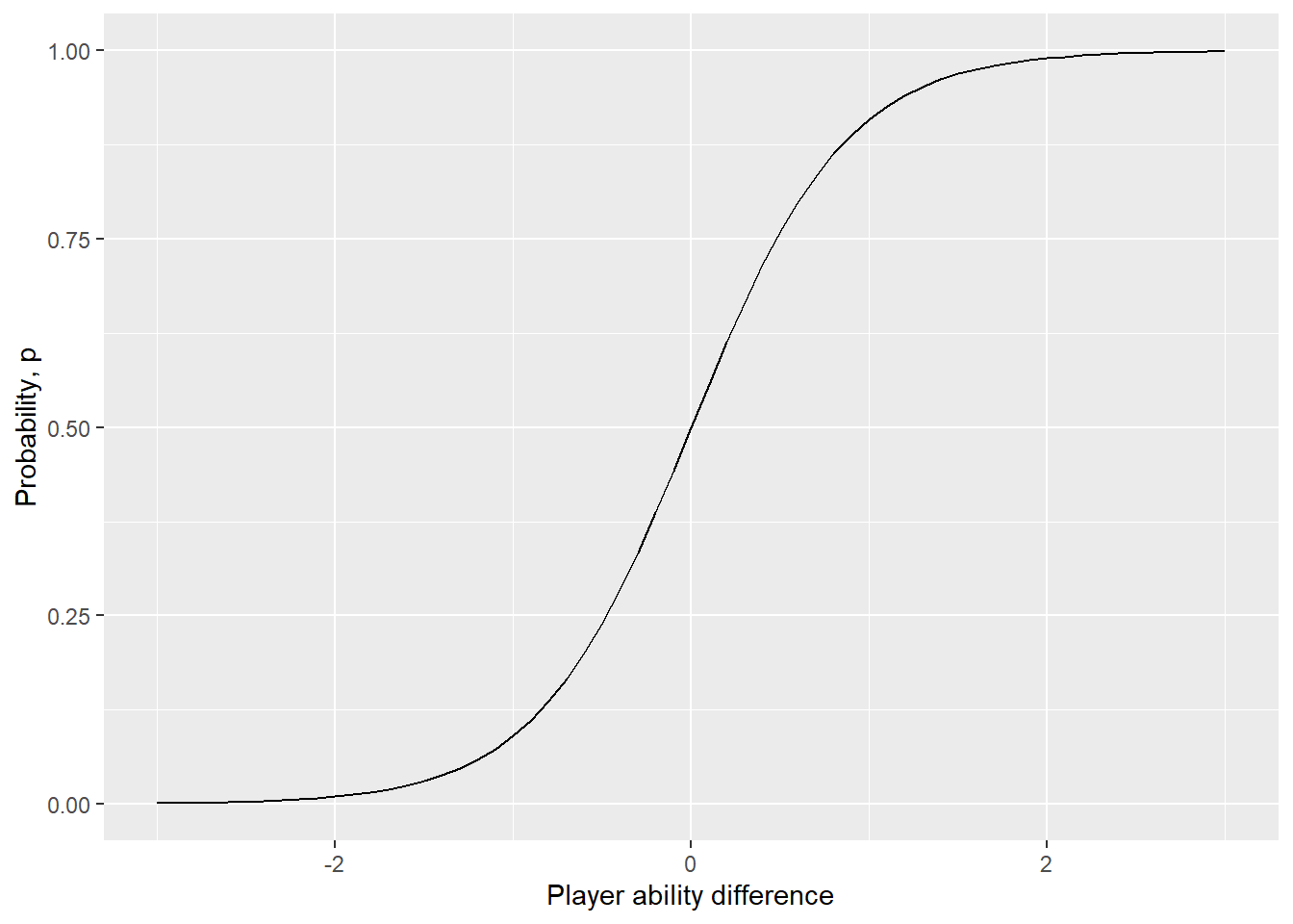
As you can see, large differenes in player abilities correspond to higher (albeit diminishingly) probabilities of winning each individual point.

Putting it all together and finding player abilities

Once we have our custom likelihood function, and our link function, it’s a simple matter of finding the player scores that maximise the log-likelihood, i.e.,

\[ \alpha = \underset{\alpha}{\text{arg max}} \sum_i P(M_i|p = \text{sigmoid}(\alpha_a - \alpha_b) ) \]

The algorithm that does this is not that important and there are many out there to choose from.

Now, I could have done this and stopped there and had a perfectly adequate rating system.

But, at the beginning of this article, I mentioned I used a Bayesian rating system, once again, taking the analysis to the next level.

Bayesian inference is a whole other topic to write about so I won’t go into details here. But, in really simple terms, Bayesian inference is a special mathematical way to use the log-likelihood from before and add on additional information (called prior information) to obtain a what’s called a “posterior-estimate”. This is an improvement on the regular maximum likelihood method in several ways:

1. We can incorporate information that we knew previously (e.g., if we knew some players are better than others without any data). Prior information can be used to essentially supplement our lack of data (recorded matches) at the beginning, thus leading to a quicker estimate of our player’s true abilities

2. The process naturally gives us credible intervals, meaning we have a degree of uncertainty about of estimates. This is because instead of finding the players’ scores that maximise the likelihood (a single point estimate), we are essentially mapping the complete posterior joint probability distribution which includes the player’s ability as parameters. Through the principle of marginalisation, we can obtain posterior probability estimates of the player’s scores. Why is this important? It’s not really its just cool. Having said, it would be important if anyone ever created a betting market in our office table tennis comp because we would be able to spot inefficiencies.

The program I used to pose and solve the Bayesian version of the above problem was Stan. Stan is one of, if not the most, state-of-the-art probabilistic programming languages out there. It has great documentation, a fantastic UI for both Python and R and a small, but growing, community. If you are looking to get into Bayesian model’s, I highly recommend giving it ago.

Admittedly, it can be daunting getting started, particularly if you come from a traditional ML or computer science background. I’m in the middle of creating some content for how to get started with Stan practically, so stay tuned. For those interested, I’ve posted the exact Stan code I used to do this in the appendix

The output of our model was the following lovely visualisation. On the top we show the current rankings complete with credible intervals and on the bottom we have a grid visualisation of who has beaten who.

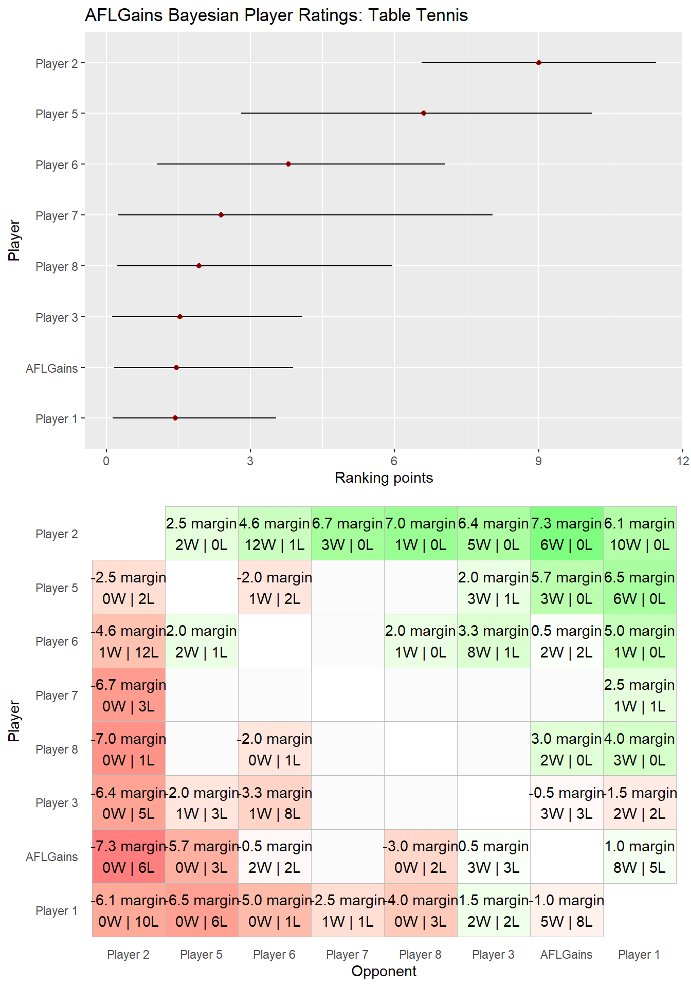
Player 2 is a clear winner having only lost once. Player 5 is an obvious second having only lost 3 times. One thing to note is that the credible interval on player 5 is much higher than player 2, because they have played far less games. This highlights the enormous benefit of doing Bayesian inference - you get a complete description of uncertainty, which is critical if you were ever to make a decision based on these results (betting for example).

Clearly, I myself am no good at table tennis. The only player I have a positive win rate over is the worst player, Player 1, although I don’t do too badly against Player 3 or Player 6.

Ironically, providing uncertainty about our player ratings has actually provided certainty that I, in fact, am not the best player of table tennis in the office. Perhaps I’ll just stick to math instead.

Appendix

// Functions used throughput the code
functions {

  //Probability of y if y < 10
  real tt_lt10(int k, real p){
    return choose(10+k,10)*p^11*(1-p)^k;
  }
  
  //Probability of y if y >= 10
  real tt_gt10(int k, real p){
    return choose(10+10,10)*p^10*(1-p)^10*p^2*(2*p*(1-p))^(k-10);
  }
  
  //Integral of win probability
  real calc_prob_win(real p){
    real win_prob;
    win_prob=0;
    for (i in 0:9){
      win_prob = win_prob + tt_lt10(i,p);
    }
    win_prob = win_prob + choose(20,10)*p^10*(1-p)^10*p^2 / (1-2*p*(1-p));
    
    return win_prob;
    
  }
  
  //Final probability mass function if y < 10
  real table_tennis_ylt10_log(int k, real p) {
    real win_prob;
    
    //win_prob = calc_prob_win(p); // actually not needed
    return log(tt_lt10(k,p));
    
  }
  
  //Final probability mass function if y >10
  real table_tennis_ygte10_log(int k, real p) {
    real win_prob;
    
    //win_prob = calc_prob_win(p); // actually not needed when calculating posterior
    return log(tt_gt10(k,p));
    
  }
  
}


// Data block to injest the data
data {
  int<lower=0> N; // Number of games
  int<lower=0> Nteams; // Number of players
  int<lower=0> team1[N]; // Player ID winner
  int<lower=0> team2[N]; // Player ID loser
  real<lower=0> prior_mu[Nteams]; //Prior for how good someone is
  int y[N]; // Match outcome (losing score)
  
  int<lower=0,upper=1> tog_dynamic;
  int game_decay_limit;
  real decay;
}

// Parameters that we need to learn
parameters {
  real<lower=0> lambda0[Nteams];
  real<lower=-5,upper=5> unit_norms[N];
  real log_process_sigma;
  real<lower=0> sigma;
  }

// Parameters that are derivatives of other paramters
transformed parameters {
  real log_lambda[Nteams,N];
  real<lower=0> lambda[Nteams,N];
  real<lower=0,upper=1> prob[N];
  
  // Initialise
  for (t in 1:Nteams){
          lambda[t,1] = lambda0[t];
      log_lambda[t,1] = log10(lambda0[t]);
  }

  // Time propogation
    for (t in 1:Nteams){
      for (g in 2:N){
        if (t== team1[g] || t== team2[g] ){
          log_lambda[t,g] = log_lambda[t,g-1] + tog_dynamic*unit_norms[g]*log_process_sigma; 
        } else {
          log_lambda[t,g] = log_lambda[t,g-1]; 
        }
        lambda[t,g] = 10^log_lambda[t,g];
      }
  }
  
  //Link function
  for (g in 1:N){
    prob[g] = inv_logit(1/10.0*(lambda[team1[g],g] - lambda[team2[g],g]));
  }
}

// Our model
model {
  //priors
  sigma ~ inv_gamma(1,1);
  lambda0 ~ lognormal(prior_mu, sigma^2);
  unit_norms ~ std_normal();
  log_process_sigma ~ normal(0,log10(1.2));
  
  //liklihood
  for (g in 1:N){
    if (y[g] < 10){
        y[g] ~ table_tennis_ylt10(prob[g]);
    } else {
        y[g] ~ table_tennis_ygte10(prob[g]);
    }

  }
}