TL/DR: I used advanced mathematics to create an alternative 2018 fixture, one that is predicted to increase total annual attendance by ~300K, while still sticking within the fixturing rules. In the article discuss how I created the solution, the final results and the impact of certain fixturing rules. Amongst other things, the study demonstrates that optimal number of Friday night matches for Carlton is indeed 5, and that the AFL foregoes ~100k per year to ensure league parity.
Introduction
Every year we wait in eager anticipation for the AFL fixture to be released. Who and when are we playing? How many games at the MCG do we have? Who has the best draw and who has the worst?
In some seasons, the fixture can be controversial. For example, in 2015, Carlton had 6 Friday night matches and most people agreed that this was a poor decision because Carlton didn’t attract crowd! A similar thing happened in 2018, where Carlton got 5 Friday night matches. This got me thinking how the fixture is actually made. Notwithstanding some strategy to give Carlton more exposure, surely in general the fixture should be scheduled such that the biggest teams that attract the largest crowds are scheduled at the right times?
In 2018, the AFL had a record 6.9M people walk through the gates over the 23 Home and Away Rounds. While this was the highest aggregate attendance in history, the situation with Carlton got me asking whether it could have been more with a different set of fixture.
In this post, I will explain how I created an alternative 2018 AFL fixture using advanced mathematical methods, with the goal to increase the overall attendance during the 2018 season. First, I’ll explain the specific set of mathematical tools I chose, the resulting fixture that was produced and then go into detail about what changed between the actual 2018 season and that suggested by the model. Lastly I’ll finish with some cool analysis and as always a discussion of what could be improved going forward.
How tough is it actually to make a fixture?
Making the fixture is hard. Really hard. To give you a flavour at just how hard, let’s think about what a fixture is. In its most basic form, a season fixture is really a collection of matches that need to decided upon, where each match is characterised by 5 parameters:
- Home team
- Away Team
- The time slot
- The round
- The ground
Let’s think about the universe of possibilities there are. We have an 18 team competition. In general, there are roughly 5 time slots (Friday night, Saturday afternoon, Saturday night, Sunday afternoon, Sunday night), roughly 10 different grounds and 23 rounds. In total, that is \(18\times17\times5\times10\times23 = 351000\) possible match definitions. Out of these universe of possible matches, we need to select 198 to make up an entire season. Some special maths (the binomial theorem) says that this means there are \(10^{733}\) different combinations of fixtures, a truly gargantuan number! To give you a rough understanding of how large this is, that is “1 with 650 zeros” times more than the number of atoms in the entire universe. And we have to choose one of them.
You might be thinking, hang on, it doesn’t seem so hard! There are plenty so why don’t we just chose one? There are two reason why we can’t just choose one of the near infinite fixture possibilities:
The rules
The chosen fixture might not be allowed. Our fixture has to abide by certain rules for it to be allowed to be implemented. For example, every team must play each other at least once. Some teams get to play each other twice, but there are restrictions on that as well. Teams can’t be on the road for too long and everyone has to have exactly one bye during the season. TV rights say you can’t have more than 3 games on Saturday night for risk of saturating the television market and you also can’t have more than 1 game on in a city at any given time-slot for risk of diluting the attendance. The list goes on. Actually there are a huge number of restrictions when thinking of a feasible AFL fixture. In fact, there are so many that only a tiny fraction of the \(10^{733}\) fixtures will actually be allowed. Now we have to wade through this massive set of fixture solutions, test them all against all the rules to find which ones would are allowed. Not an easy task.
The benefit
Let’s say we somehow landed on a fixture that works, how do we know it’s any good? What do we even mean by good? Well, we know that it’s good because it abides by all of our rules. But is that the best we can do? What about if there was another different fixture that also was allowed by our rules, but meant that teams had to travel less in aggregate? Wouldn’t that be better?
In general, simply choosing a fixture that is feasible isn’t enough - we would like a way to obtain the best fixture possible. That is, we would like to optimise our fixture, which means we need to evaluate all the feasible ones and chose the best one. Again, not an easy task
So how could we possibly do this? The answer is to use a special branch mathematics called linear programming.
Linear programming
Linear programing is an advanced mathematical technique that has been around for decades and was introduced to solve the following problem: if I have a bunch of decisions I have to make, with a clear measurable goal I’m trying to achieve and clear rules that I need to stick to, tell me the decisions that I need to make in order to get me closest to my goal without breaking any rules.
This looks like our AFL fixturing problem. We have a number of decisions we need to make (which combination of matches will we choose), with a whole bunch of rules that restrict how these decisions are made (TV rights, number of home ground games, number of matches played in a city at any given time etc..). The last thing we need is some sort of fixturing goal. For us, we’ve chosen the total attendance across the season, so we need some what to relate our chosen match to a predicted attendance. We’ll get to that in a bit, but for now it is clear the linear programming is the tool we want.
A bit more on linear programing for those who are interested. It’s often used in the manufacturing world to make decisions on when to make certain products, where and how much to send on trucks and which warehouses / factories to open or shut-down to maximise profit or minimise cost. It works by allowing you traverse to space of possible solutions in a really efficient way so that you can get to the optimal solution in a fraction of the time it would take you to go through and evaluate each solution individually. For this reason is truly is one of the most powerful and valuable applied mathematical techniques ever developed.
Formulating the problem (this gets maths heavy so skip to the next section to see the results)
So we know we want to use linear programming. How can we use it? Well, whenever we want to use linear programing, we need to write down our specific problem as a series of mathematical equations. This series is known as the “program”. This might sound daunting or even impossible, but luckily there is a standard and simple 3 part framework that we can apply to make things easier.
Our decisions
We’ve actually already talked about this before. Our decision is which matches to use, where each match is comprised of 5 parameters: home teams (i), away team (j), time slot (t), ground (g) and round (r). Let us define a 5 dimensional binary variable (binary means 0 or 1), called \(\chi(i,j,t,g,r)\), as a function of these 5 parameters. \(\chi = 1\) if we decide to use that match in our schedule, while \(\chi = 0\) if don’t decide to use it.
As a concrete example, the first match of 2018 season was: Richmond vs Carlton at MCG on Thursday night in Round 1. In the way we have defined it, we would express this as
\[\chi(\text{Richmond}, \text{Carlton}, \text{Thursday Night}, \text{MCG}, \text{Round 01}) = 1\] To reiterate, with linear programming we don’t specify which \(\chi\)’s are 1 or 0. We let the computer decide. We just define the rules around making this decision.
Our rules
Thinking of all of the possible rules that existed in the fixture was the hardest part of this whole exercise. There are some rules that exist online here and other rules that are really obvious (you can’t play more than once per round for example). The really hard rules are the ones that aren’t obvious and must be inferred from staring really hard at the current fixtures and thinking really hard. Below is a list of rules that went into the final model:
- Every team can play maximum once per round
- Every team must play every other team at least once
- Every team must play every other team no more than once at the same home ground
- There can be at most one match on Thursday or Friday every round
- Every ground can only host one match at a particular day and timeslot
- Each team must play a total of 22 matches
- Each team cannot travel more than 2 weeks on the road
- Adelaide Oval must have at least 22 home matches
- SA, NSW, QLD and WA cannot have more than 1 match per round
- Bye Rounds must occur between round 7 and round 15
- Victoria cannot have more than one match per time slot
- MCG cannot have more than one match per day
- There can be no more than 3 Saturday night matches
- Sunday must have at least 2 matches and no more than 3 matches
- All teams must have 11 home matches
- All equity contraints must be adhered to
- The season must include the following special matches
- Port and Gold Coast play in China in Round 9, with a bye happening in Round 10
- Collingwood and Essendon play at the MCG in Round 5 on Wednesday
- Melbourne and Richmond play at the MCG in Round 5 on Tuesday
- Melbourne and Collingwood play at the MCG in Round 12 on Monday
- Essendon and Richmond play at the MCG in round 11 on Saturday
- Gold Coast and Freo play at Perth stadium in Round 3 as Gold Coasts home game
- The season must include the following contractual agreements:
- GWS must play at UNSW 3 times
- Bulldogs must play at Mars stadium 2 times
- Kangaroos play at Bludstone arena 3 times
- Hawthorn play at UTAS 4 times
- Gold Coast play at Cazaly Stadium once
- Melbourne play at TIO stadium 2 times
I’m sure there a few rules that I’ve missed. One particular one that comes to mind is that Gold Coast Suns weren’t allowed to play at their home ground for the first 10 rounds of the season. Nevertheless, the list of probably comprehensive enough to give us an 80-=90% good enough solution.
Each of these rules needed to be translated into mathematical form. While I won’t go through all of the rules, I’ll give one as an example. One of the rules states that each team can only play maximum once per round. Mathematically, this would be described as:
\[\sum_{j,t,g} \chi(i,j,t,g,r)+\chi(j,i,t,g,r) <=1 \space \forall \space (i,r) \]
To translate, this says that for each round (\(r\)) and each team (\(i\)) the sum over all grounds (\(g\)), timeslots (\(t\)) and opponents (\(j\)) for both home games (\(\chi(i,j,t,g,r)\)) and away games (\(\chi(j,i,t,g,r)\)) must be less than or equal to 1.
Our goal
I’ve assumed that the goal of the fixture is to maximise total attendance. This assumption is probably reasonable, but there are of course other strategic business objectives. These might include, for example, growing the game in low penetration areas such as Tasmania. Where possible, these strategic goals are taken into account in the form of decision rules (for example we have said that Hawthorn must play 4 home games at UTAS).
Like our constraints, our objective function needs to be expressed as a mathematical equation. Let’s say that the attendance for each game is represented by \(A(i,j,t,g,r)\), where parameters \((i,j,t,g,r)\) define the match. So our objective function would look something like:
\[\text{Total Attendance} = \sum_{i,j,t,g,r}A(i,j,t,g,r)\chi(i,j,t,g,r)\]
So how do we tell how much attendance will be for a given match? This is where predictive modelling and linear programming meet each other. In a previous post, I discussed how I used various factors to predict the outcome of AFL matches before they had started. We can use a similar approach to try and predict the attendance of a match for a given set of teams.
To build the predictive model, I scraped data attendance data from the year 2000-2017 from AFL tables and used a technique called linear regression to relate various input features with the attendance. The output of linear regression gave us the following equation:
\[ \begin{aligned} A(i,j,k,g,t)=\\ -283+\\ 2168\times(\text{State is NSW})+ \\ -7.8\times(\text{State is Qld})+ \\ 4759\times(\text{State is SA})+ \\ 2619\times(\text{State is Vic})+ \\ 5473\times(\text{State is WA})+ \\ -4865\times(\text{State is Other})+ \\ 299\times(\text{Time is Saturday Night})+ \\ -1319\times(\text{Time is Sunday Afternoon})+ \\ -1831\times(\text{Time is Sunday Night})+ \\ 3443\times(\text{Time is Thursday or Friday Night})+ \\ 0.1529\times(\text{Ground Capacity})+\\ 0.6257\times(\text{Average Attendence between teams})+\\ 0.0652\times(\text{Home game membership})+\\ -1744\times(\text{Greater than Round 16})+\\ -631.2\times(\text{Between Round 6 and 15})\\ \end{aligned} \]
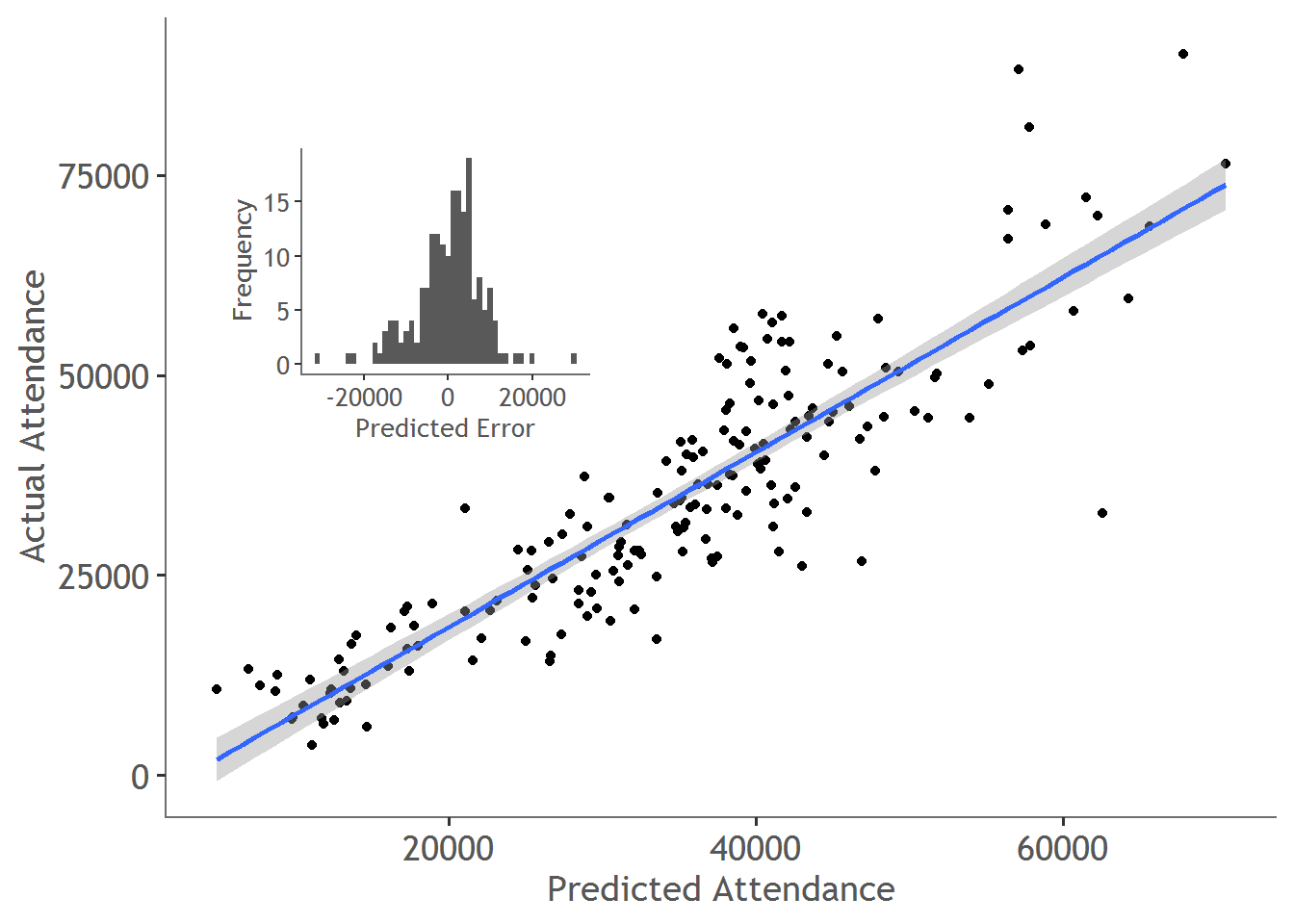
The model was then tested on 2018 data and achieved an \(r^2=0.78\). The performance of the model can be visualised by plotting each matches predicted attendance with their actual attendance. As we can see, the model does a good job at predicting overall attendance. To ensure that there were no biases in the model, we can look at the distribution of error. The distribution forms a nice normal (like) distribution, indicating a reasonably unbiased model.
Solution method
Now we have all of the ingredients that an optimisation problem needs: Some concrete decisions, some rules formulated as mathematical expressions and a goal mathematically linking the decisions to what we would like to optimise. So how do we solve it? Well, basically what we have to do is write down all of the equations in a special computational solver and let the computer figure it out. There are lot’s of solvers out there on the Internet which employ special algorithms to get to an answer. These algorithms include the Simplex method, cutting planes or branch and bound. The solver I used was called CPLEX 12.8 and after I wrote down all of the rules into the solver, the whole problem took about 3 hours to run on my laptop.
When implementing the program, I had to make a few simplifications. For each day I split the fixture into either ‘early’ or ‘late’ depending on whether the match starts after 4 pm or not. When using the results, the idea would be that the exact time would depend on contractual agreements with the grounds. I also combined the timeslot Thursday and Friday night into one time slot called “ThursdayorFridayLate” and allowed up to 2 games to be played during this time. For situations where there are two matches scheduled to be played on this day, we would simply randomly allocated Thursday or Friday to each of these matches respectively. I don’t expect these simplifications to meaningfully change the the result.
Results
The full optimal fixture can be found here. Below is a table summarising the key metrics of the new fixture.
| Team | No. of Home Games | No. of MCG games | No. of Thursday/Friday Night Matches | No. of Sunday Matches | Bye Round | Predicted Attendence (k people) |
|---|---|---|---|---|---|---|
| Adelaide | 11 | 2 | 0 | 3 | 16 | 485 |
| Brisbane | 11 | 2 | 2 | 0 | 15 | 234 |
| Bulldogs | 11 | 2 | 4 | 3 | 14 | 351 |
| Carlton | 11 | 14 | 5 | 5 | 16 | 507 |
| Collingwood | 11 | 13 | 4 | 2 | 14 | 555 |
| Essendon | 11 | 15 | 2 | 6 | 16 | 554 |
| Freo | 11 | 4 | 4 | 3 | 15 | 429 |
| GCS | 11 | 3 | 1 | 3 | 10 | 138 |
| Geelong | 11 | 5 | 6 | 1 | 09 | 400 |
| GWS | 11 | 2 | 0 | 4 | 16 | 136 |
| Hawthorn | 11 | 8 | 3 | 3 | 09 | 521 |
| Kangaroos | 11 | 5 | 3 | 1 | 16 | 339 |
| Melbourne | 11 | 12 | 1 | 3 | 16 | 429 |
| Port | 11 | 2 | 1 | 2 | 10 | 444 |
| Richmond | 11 | 16 | 4 | 1 | 16 | 535 |
| StKilda | 11 | 2 | 3 | 0 | 16 | 364 |
| Sydney | 11 | 5 | 0 | 3 | 11 | 337 |
| WestCoast | 11 | 4 | 3 | 3 | 11 | 463 |
Well, I wasn’t expecting that. The optimal number of Friday / Thursday night matches for Cartlon is 5! Sorry guys, I take back everything bad I said about Carlton!
When you think about it though, this actually makes a lot of sense. When you look at the equation for attendance, Friday/Thursday night matches have the highest attendances in general, compared with other time slots. So by scheduling ‘smaller’ teams that typically attract less people, you are avoiding greater losses that you would otherwise incur by scheduling them elsewhere, ensuring that the total attendance for the league is higher.
The total attendance is 7.22M, 0.32M more than the actual attendance for 2018. That is a substantial number of extra people. Let’s assume the AFL gets something like 20 dollars per additional person (since all fixed costs of renting the grounds are already paid for). That’s an extra $6.4M of straight profit. This could be portioned out to the clubs to prevent them from resorting to other income streams, such as pokies.
Let’s have a look at the round by round attendance uplift (the baseline 2018 fixture can be found here ) 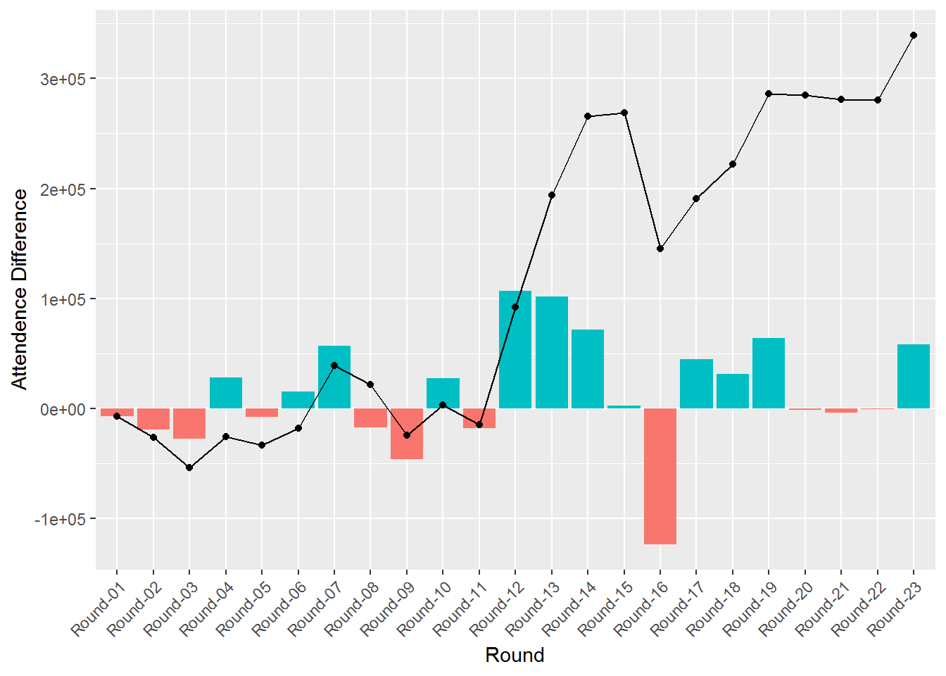 Most of the gains come from the middle of the season. In some rounds we actually incur a substantial loss. In the next section, we will discuss 1) how this loss is a necessary penalty due to inherent trade-off’s in the problem and 2) how optimizer reconciles these trade-offs.
Where is the extra attendance coming from?
Trying to understand the results of computational optimisation is really hard because unlike a human, the computer considers all possible positive and negative outcomes simultaneously for every descision, including all flow-on effects. Sometimes these flow-on effects can only have positive benefits really far down the chain, so it’s not at all obvious why a certain decision was made. In practice, the best we can hope for is to compare the baseline and optimal solution and look for systematic patterns.
To do this, we’ll define a simple frame-work for investigating the change between the baseline and optimal fixtures. It turns out that the difference between any two fixtures can be described completely by a collection of 4 different types of alterations:
- A simple change - Where the home and away team remain the same but the time slot, round and ground are changed
- A swap - Where the home and away teams are reversed and the ground is changed. The timeslot and round are also changed.
- An addition - Where a game is added where it didn’t exist before
- A subtraction - Every additional game must be followed by a subtraction somewhere else..
It also turns out that when we perform an alteration, we are creating (or removing) attendance using one or more of five different attendance drivers (These are actally the different components of our linear regression model):
- A State change - Describing the accessibility of football and willingness to attend in a particular state
- Time slot change - Describing the willingness of people to attend at a particular time.
- Seasonal change - Describing the willingness of people to attend during a particular point in the season
- Membership change - Describing the expected amount of people attending due to the size of the home team’s membership.
- Capacity change - Describing the expected amount of people attending due to the size of the ground
For example, let’s compare the GWS Freo game in both scenarios.
| Scenario | Home | Away | Ground | Timeslot | Round | Predicted Attendance |
|---|---|---|---|---|---|---|
| Baseline | GWS | Freo | UNSW | Saturday Afternoon | 4 | 12106 |
| Optimal | Freo | GWS | Perth Stadium | Saturday Night | 12 | 38437 |
This change is a “swap” since the home and away team and swapped positions. According to our model, this swap will result in 26330 more people attending the match. The 26330 can be broken down in the following way:
| Attendance Driver | Value |
|---|---|
| State Change | 3305 |
| Time slot change | 299 |
| Seasonal Change | -631 |
| Membership change | 16254 |
| Capacity | 7103 |
| Total | 26330 |
We can see that moving the the match to WA will increase attendance because the ground is larger, the home team has more members, and the state is more able and willing to watch the match. There is also a small jump in attendance due to the timeslot shifting from afternoon to night. Interestingly, the model has chosen to sacrifice some attendance by shifting to later in the season, presumably because it’s winter and on average, attendance tends to reduce during winter. However, this sacrifice is overshadowed by the total gain from the other drivers, hence the swap makes sense.
It should be mentioned though that because we are swapping out a home game from GWS, we will need to swap or add another home game from GWS somewhere else down the line. This will have a ‘flow-on’ effect and alter attendance numbers somewhere else in the chain of matches. The alteration will subsequently alter other matches and so on and so forth. The power of the linear optimisation is that it is specifically designed to take all these possible alterations and flow effects into account.
In total, there are 210 separate alterations that happen. You can find a breakdown of those alterations here. Let’s now see the overall breakdown of attendance changes:
| Value Lever | State | Capacity | Timeslot | Season | Membership |
|---|---|---|---|---|---|
| Add/Delete | -1093 | 68062 | -3445 | 9683 | 39000 |
| change | 0 | -25012 | 53756 | -10614 | 0 |
| swap | 1093 | 44426 | 30067 | 5382 | 127749 |
This table is telling us that the primary lever that is being pulled to increase attendance is swapping, the mechanism we discussed as our example. The optimizer tends to swap games around (where possible) so that larger teams play at the largest grounds, utilizing better timeslots, better capacity of the ground and, most importantly, taking advantage of the home team’s larger attendance base.
The good thing is though, that this doesn’t occur in isolation. Games and changed, added and deleted in response, so that the solution can feasibly swap games but still stay within the rules of the fixture. Sometimes this happens with a negative effect on attendance, but overall the changes are being made for the holistic benefit of the fixture.
For example, like the Freo-GWS game, the Richmond-GWS game is also changed from Spotless stadium to the MCG. To allow this, the Richmond-Brisbane Game is changed from the MCG in Round 4 to the MCG in Round 14, where it actually net loses 600 people due to the impact that the time in the season has on average league wide attendance.
How much better is our solution really?
We now have a solution that has the potential to increase attendance by about %5 over our current baseline. But how large is this really? For this we need to get a sense of good our current solution is. One way to do this is to compare both the baseline and optimal solution to the worst case scenario. That is, a fixture that purposely tries to minimise attendance.
In mathematical terms, we can do this by simply flipping the sign of our objective function, i.e., rerunning the optimization trying to maximise negative attendance. Here is the result.
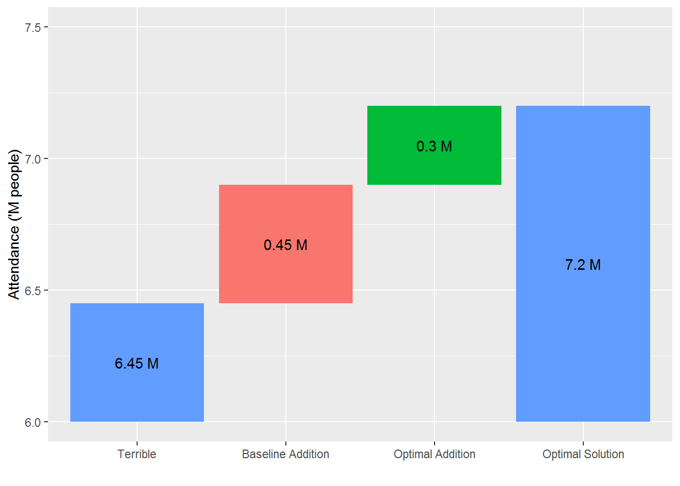
As we can see, the ‘terrible’ fixture has a total attendance of 6.45M. It’s a terrible fixture, but one that is theoretically allowed. It chooses to do silly things like always using the Sunday time slot and scheduling Hawthorn and West Coast at UTAS. The current 2018 fixture is a whopping 450,000 people (8%) higher the worst solution. Clearly some kind of attendance maximisation is going on at AFL and they have done a really good job. However, the potential optimal solution adds an extra 340k on-top of this 450k. In relative terms that 75% more uplift!
Using this anlaysis, I think it’s safe to say that the AFL could have broken the 7M mark quite easily with a better fixture that still adhered to all of the fixturing rules
The cost of equality
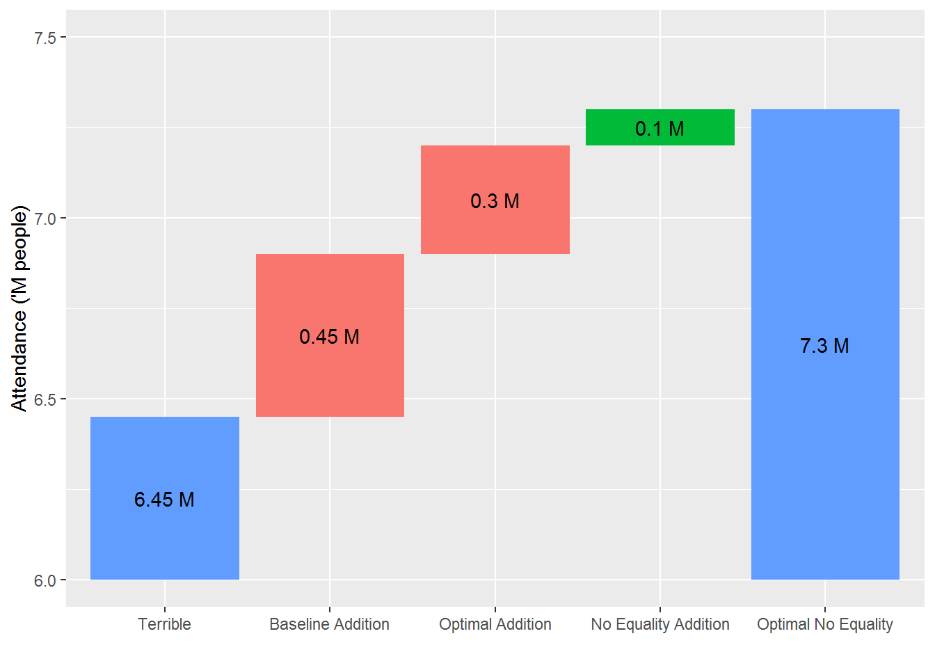
One truly awesome feature of linear programming is that it guarantees to give you the optimal solution for a given set of rules. This means that if we took certain rules away it would give us a different solution. This solution will actually be a more valuable fixture (in terms of attendance), since it is less restricted. We can use this concept to our advantage. Let’s see what happens when we remove all of the “equality” constraints (those constraints that say ‘hard teams’ have a harder fixture than easier teams and are explained here ).
The figure below shows the cumulative attendance for a best fixture possible when we remove the equity constraints. As we can see, the benefit over the current optimal solution with equity restrictions is around ~100k people. What this is actually telling us is the opportunity cost of the equity constraint. That is, the AFL loses 100k potential customers by attempting to ensure parity in the league. So now we know the price the AFL pays for its efforts to ensure parity.
On this note, its important to note why a 23 round fixture is actually good. Having the ability to schedule some teams to play each other twice gives us a larger mechanism to ensure difficulty differences in the fixture. And this is done to ensure that lower placed teams in on year have a greater chance of making the finals than those who did so last year, thereby enforcing a level of parity in the league.
Improvements
As with any investigation, things could be improved. There are certain constraints that I didn’t put in, either because I’m lazy ( I did this in my free time) or because they would have made the solution too computationally expensive.
One constraint that comes to mind is the requirement for GCS to not play at Metricon for the first 10 rounds of the season.
Another constraint that I left out is the requirement that teams have roughly the same number of days rest between matches, give or take one day or so. This means that if you played on a Sunday, and then played on the next Friday, your opponent cannot have played on the last Friday, because they would have had 2 more days rest than you.
However, in general the time slot value driver is small when compared with the other value drivers. So there is always the possibility of taking the current optimal solution and manually tweaking it so that the rest days are aligned. Although I don’t know for sure, my hypothesis would be that the attendance lost due to timeslot shuffling would be minimal.
Conclusion
Now let’s summarised what we’ve talked about in this (rather long) article. In essence we used a branch of advanced mathematics called linear programing to create alternative AFL fixtures, specifically designed to maximise attendance. We used a regression model to relate typical match descisions with predicted attendance and used this as the goal function in our optimisation. We inferred the fixturing rules by looking really hard at the current fixture. Finally, we obtained a solution by using CPLEX 12.8.
From looking at the difference between the optimal fixture and the baseline we came to a number of conclusions:
- The optimal number of Friday / Thursday night matches for Carlton is 5!
- It’s probably safe to say that the AFL could have broken the 7M mark quite easily with a better fixture that still adhered to all of the fixturing rules
- The current AFL fixture is quite good with respect to the worst possible fixture that’s possible
- The AFL loses ~100k potential customers by attempting to ensure parity in the league.