TL/DR: I made a machine learning algorithm to predict AFL matches before they started. When I simulated my results on 2017 matches and used it for betting, I managed to get a net positive return on my investments.
Introduction
A few months ago I posted an article introducing the concept of machine learning in AFL. You can find that article here [https://www.aflgains.com/2018/04/25/machine-learning-in-afl-part-i-does-the-free-kick-differential-really-matter/]. I presented some use cases about where it could be practically applied, including injury prevention and management, drafting, in-game strategy and strategic trading. These use-cases were all geared toward benefiting the club. There is, however, one area that machine learning excels at that would benefit punters and tippers - game prediction: predicting the outcome of a match before it has started. In this article, I will focus on how I built a machine learning model to do exactly that.
This article is structured as follows: first I will briefly describe supervised machine learning. Next I’ll move into how I created the model to predict AFL matches- I’ll discuss the data, features and methodology that I used. I’ll then discuss the final results including accuracy, potential improvements and, most importantly, how to use it to make money.
Supervised machine learning
Supervised machine learning is probably best understood in an AFL context with a simple example. Suppose we wanted to predict the outcome of a particular match. We don’t know anything about AFL, but we have a friend that has presented us with some historical matches and we have found a pattern that the home team tends to win more often than the away team. So we pick the home team.
What we have just done is created a very simple “model” (a mental model in this case) to predict the outcome of a match based on previous experience. In our data we have only used one data “feature” - the home/away status of the team. In fact, using this one feature, we would have an expected accuracy of 58% because the home team wins 58% of the time.
At this point it is useful to define a few terms:
- Prediction: The best guess for the outcome of a match e.g., win/lose
- Feature: the information that we use the make a prediction, e.g.,. home/away status
- Model: The relationship between the feature and the prediction e.g., if home then win otherwise lose
Now, we want to improve our prediction accuracy by introducing more features. This means we start to ask other questions about the teams and the conditions. For example, what is the weather like? Who are the key players that are included in each squad? What are the respective ladder rankings? What are the historical outcomes between the two teams?
Now these combination questions are getting more and more difficult to answer using basic intuition. For example, we might notice that teams with higher contested possession win more often. But what happens then when the team with a higher historical contested possession count is the away team? How much contested possession differential outweigh home ground advantage? What is the trade-off?
This is where machine learning will help us. Basically it is a mathematical technique that can automatically map the relationship between features and predictions using historical observations. It will “learn” the statistical trade-offs between contested possession, homeground advantage and any other relevant features to help use make a prediction about the game outcome.
Other than sports, it’s applied in many industries including real estate (to predict a house price), banks (to predict whether someone will default on a loan), internet advertisements (to predict whether someone will click on an ad if presented), Google (to predict if your picture has a cat in it) and many more.
Creating a machine learning model to predict AFL matches
What was the goal?
I tried to predict the outcomes of the 198 matches played in the 2017 AFL Home/Away season using data only available on AFLTables.com.
A little bit about the AFL 2017 season - this season is notorious for being one of the most even in history. In fact several posts were written about this on Reddit [https://www.reddit.com/r/AFL/comments/6ls48y/this_is_the_most_even_season_since_1998/] and some articles even were written in the paper [https://www.theaustralian.com.au/sport/afl/afl-2017-most-even-comp-since-expansion/news-story/b3a15b2ad17fe9727244c19aecbc01d2]. This means its one of the most difficult to predict.
What data was used?
The data used for the study was web-scraped from AFLTables.com and contained all in game player information from 2003-2017. This constitutes approximately 2700 individual matches and contains data on key player statistics and venue of game played.
What features were used?
The features (information) that I used to try to predict matches can be classified into 6 broad categories. For each game (combination of home and away team), we can calculate difference in team ranking, form line, venue experience, key game statistics, player ranking and line up and fatigue.
1. Team ranking:
This was simple the different in ladder position, difference in number of ladder points, and difference in rolling 5 game percentages.
2. Form-line
This was simply the difference in the win-loss record over the last 5 rounds.
3. Venue experience( Home ground advantage or HGA):
This was the difference in wins at a particular venue between the home and away team over the last two years
4. In-game Statistics differential
These are the differences in in-game statistics between the home and away team, averaged over the last 5 rounds. These include: win loss form, score, percentage, kicks, handballs, contested possession, tackles, hit outs, rebound 50’s, inside 50s; free-kicks, clangers, marks inside 50’s, goal assists, bounces, time-on-ground.
Along with differences in the mean, the difference in the variance variance was also taken into account.
5. Player information
Along with team statistics, player performance was also taken into account. I used u’s player rating formula and took the average player rating over the last 5 rounds. I then looked at the line up and based on the average player rating over the last 5 rounds for each player, calculated the expected total player rating for the upcoming match.
6. Team information
I also looked into team line-up before the match. For each match, I calculated the top performer for goals, clearances, goal assists, tackles, contested marks, and rebound 50s for the last 5 matches for both the home and away and determined whether or not that player was playing in the current match.
7. Fatigue
I modeled a fatigue factor as which third of the season we are in (1-8 = Beginning, 9-16 = Middle, 17-23 = end). I also had a feature in there indicating whether it was Round 1 or not so that the machine could learn any differences between round 1 predictions and the rest of the season.
How did I assess the model?
I used “accuracy” as our simple measure of performance. This is defined as the total number of correct guesses divided by total number of matches. E.g., If I had 120 correct guesses my accuracy would be 120/198 = 60.6%
What was the model?
This is a little technical so feel free to skip to the next section
The data was partitioned into a validate/train set (Season 2016 and below) and a hold-out set (being 2017 season).
I used an Extreme Gradient Boosted Model and optimized it’s hyper parameter using grid search with 5-fold cross validating (using randomly selected validation set). After the hyper parameters were chosen and finalised, the 2017 matches were predicated.
To generate confidence intervals in the predictions I trained 99 more models on bootstrapped versions of the data.
Results
Final accuracy
The final accuracy of the model was 66.7%.
66.7% sounds low, but is it really that low? To benchmark these results, I downloaded some published tipping results from “experts” (after the H/A season had finished) from the herald sun. I also calculated the accuracy of what you would have achieved had you followed other stats related methods including the betting odds (http://www.aussportsbetting.com/data/historical-afl-results-and-odds-data/), the Swinburne Computer (https://www.swinburne.edu.au/footy-tips/2017-footy-tips/) and simply tipping the home-team.
| Rank | Tipster | Total |
|---|---|---|
| 1 | Chris Cavanagh | 135 |
| 2 | Trent Cotchin | 133 |
| 3 | AFL_gains tipping machine | 132 |
| 3 | Gerard Whateley | 132 |
| 5 | Odds | 131 |
| 5 | Lauren Wood | 131 |
| 7 | Tim Watson | 128 |
| 8 | Michael Warner | 127 |
| 9 | Jon Anderson | 126 |
| 10 | Swineburne Computer | 125 |
| 10 | Mark Robinson | 125 |
| 12 | Matthew Lloyd | 124 |
| 13 | Sam Landsberger | 122 |
| 14 | Bianca Chatfield | 121 |
| 14 | Jay Clark | 121 |
| 14 | Patrick Dangerfield | 121 |
| 14 | David King | 121 |
| 14 | Glenn McFarlane | 121 |
| 14 | Rebecca Williams | 121 |
| 20 | Kevin Bartlett | 120 |
| 20 | Sam Edmund | 120 |
| 20 | Jon Ralph | 120 |
| 20 | Malcolm Turnbull | 120 |
| 24 | Eliza Sewell | 119 |
| 24 | Bill Shorten | 119 |
| 26 | HomeTeam | 118 |
| 26 | Scott Gullan | 118 |
| 28 | Mick Malthouse | 117 |
| 29 | James Hird | 116 |
| 30 | Dermott Brereton | 115 |
| 30 | Gilbert Gardiner | 115 |
| 32 | Marcus Bontempelli | 114 |
| 33 | Scott Pendlebury | 110 |
| 34 | Kiss of Death | 74 |
The model comes equal third, only behind Chris Cavanagh and Trent Cotchin. It out performs, most experts, the Swinburne computer and outperforms betting odds. Special shoutout to Scott Pendlebury, Marcus Bontempelli, James Hird and Mick Malthouse who notibly did worse than simply tipping the home-team.(this is potentially due to team bias for the players…).
What is important to predict match outcomes?
We can use a technique called variable importance to understand which features the model thinks is important to consider when making predictions, and which features aren’t important. This is presented as a rating between 0 and 100, where 100 means very important and 0 means not important at all.
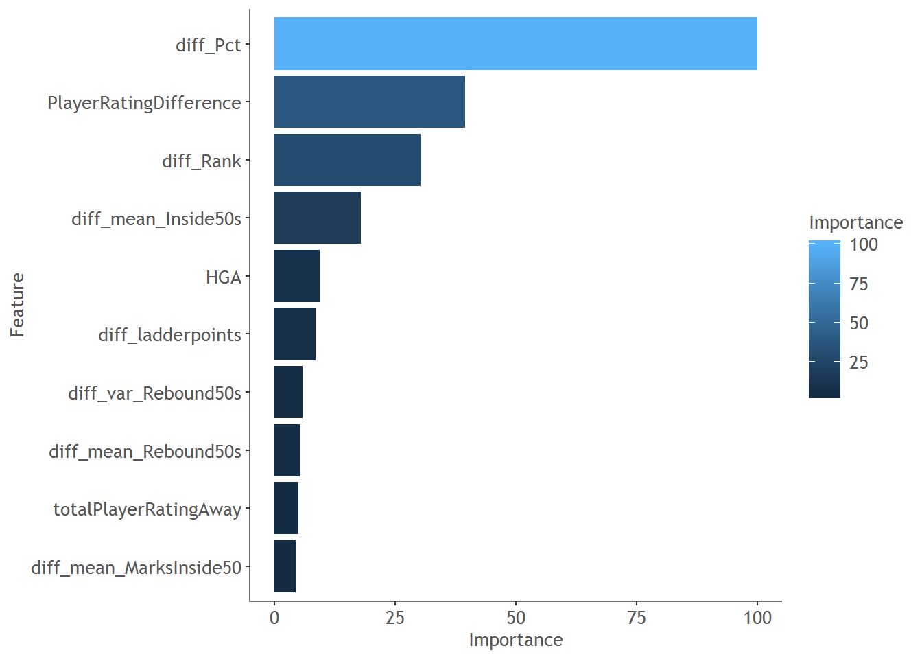
Here are the relative ranking of the top 10 features. Surprisingly, the largest driver of a win is actually the difference in the 5-game rolling percentage. The other features that are important are ones you would expect: player performance, ranking and home-ground advantage. Of the actual in-game statistics that make a difference, inside50’s and marks inside 50s appear to be the most predictive.
Using the model for betting
And now for the most important question - could I have used this model to make money on the betting markets?
The short answer is … I would have, but this may just be luck.
Here is a graph the ranks each of the 198 matches of the home and away season based on the probability of a home win. The grey bars are the 90% confidence on that probability. For example, for the first point, we estimate the probability of the home team winning is about 88-93%. The triangles are the corresponding probability of the home team winning as given by the betting odds (if you didn’t know 1/Price of the odds gives you the probability, so if the home team are paying at $1.37 they are valued at 73% likelihood of winning).
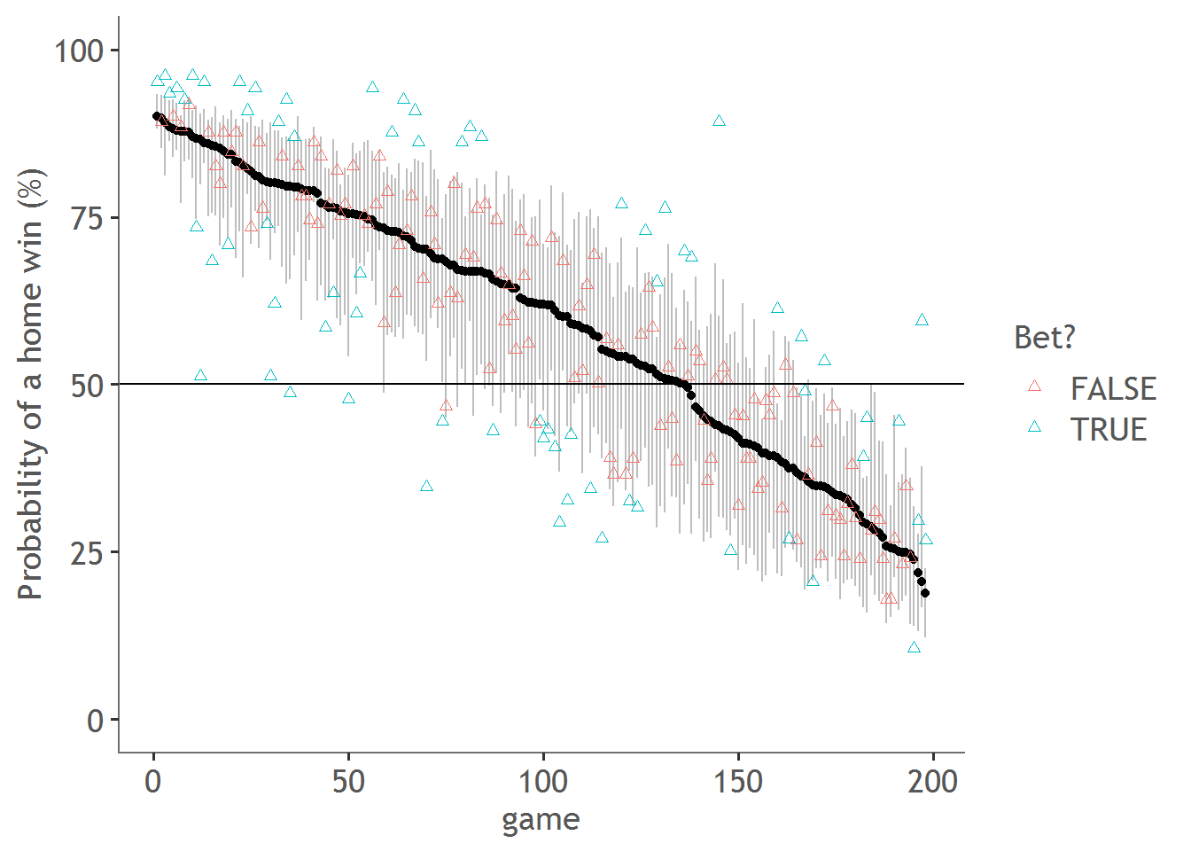
To put it short, red triangles are games where the predicted probability is similar to what our model estimates because they fall within the confidence bands. Blue triangles are those that we think have been sufficiently miss-predicted and therefore we spot an opportunity to place a bet.
So, for every game with a blue triangle I placed a (virtual) bet of 100 dollars. If the 5th percentile home probability was higher than that given by the odds, I bet on the home team (because the home team was overvalued). If the 95th percentile was lower than that given by the odds, I bet on the away team (because the away team was overvalued).
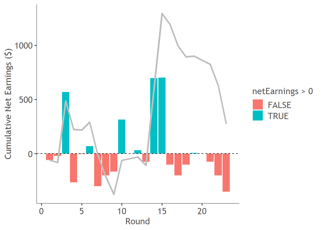
Here is the round-by-round cumulative winnings. In total I won a net $275 from a total investment of 6900 dollars - an absolutely massive ROI of 3.9855072%.
Can we do any better?
We can also visualise the winnings on the same graph as before - here I’ve placed an ‘X’ for games I lost money and a green square for games I won money. The size of the green square is proportional to the amount I won.
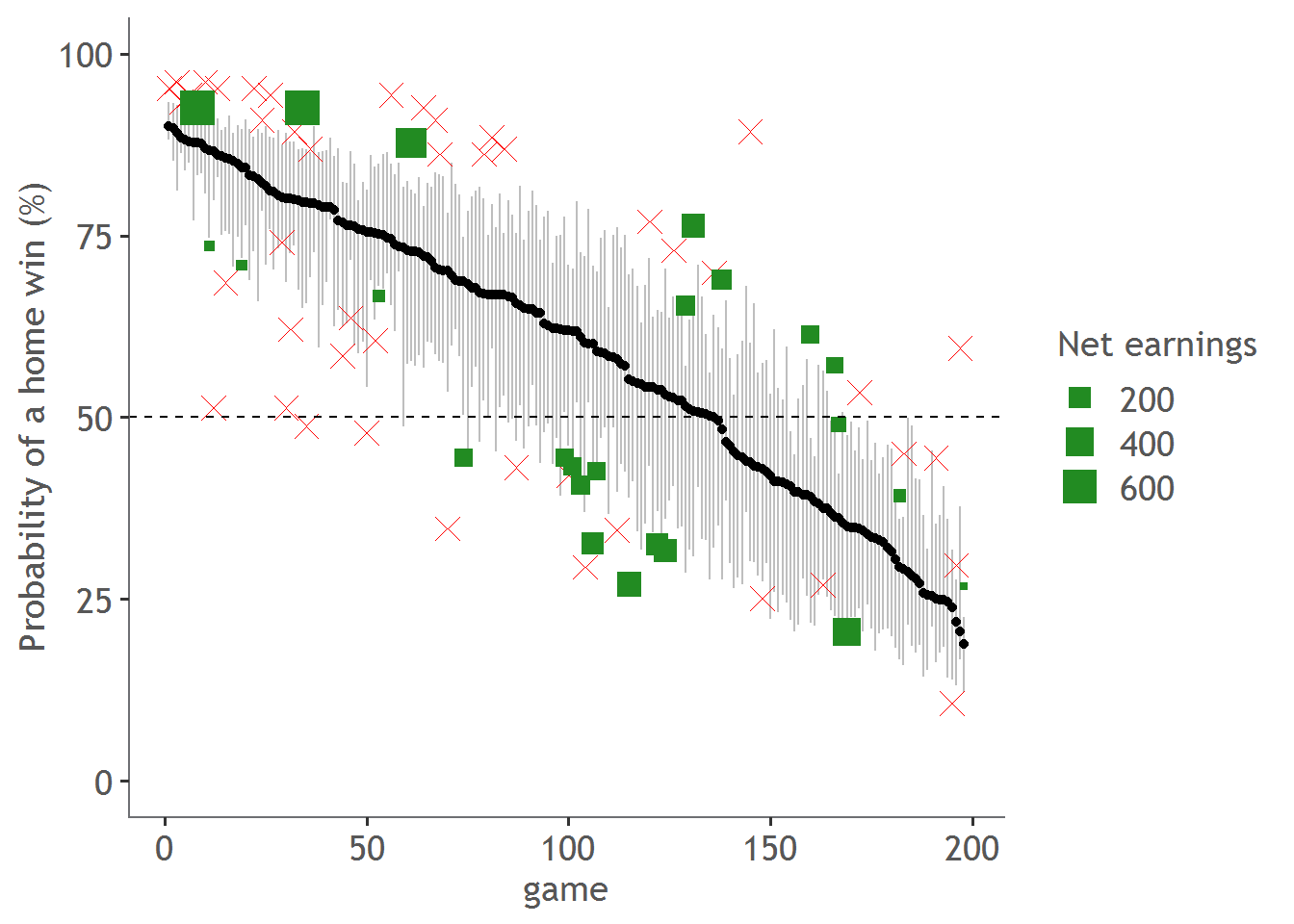
This visualise shows something interesting…there appears to be a 4 separate clusters of points, one in each corner of the graph. Here is the graph again with those clusters shown:
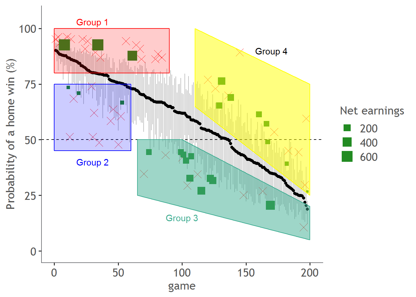
Group 1 (red) are games where the home team is expected to win but by too much, group 2 is where the home team is expected to win but by not enough, group 3 (green) is where the home team is expected to lose but by too much, and group 4 (yellow) is where the results appears 50/50.
If we analyse each of these groups for their expected winning probabilities (as per the odds), the actual winning percentages and total net earnings we see something very interesting.
| Group | Net Earnings ($) | Expected Win (%) | Actual Win (%) | No. of Games |
|---|---|---|---|---|
| 1 | -52 | 91.71 | 85.71 | 21 |
| 2 | -873 | 61.37 | 23.08 | 13 |
| 3 | 1149 | 33.68 | 55.56 | 18 |
| 4 | 51 | 57.97 | 52.94 | 17 |
Group 1 and 4 tend to have very low net earnings. For these groups we are winning as much as we are losing, so our model and the Odds are at a stalemate. According to our model, the Odds have over valued the home team, but our model doesn’t consistently identify this opportunity correctly to create a positive net yield.
Conversely, (and rather strangely) there is Group 2, where both the model and the Odds do a terrible job at predicting the home win. In fact, the expected winning percentage (according to the Odds) for Group 2 is 60% compared with the actual winning percentage of 23%!. The reason why we lose money in this case is that while both models do a terrible job, the odds are slightly less terrible.
Finally, let’s look at group 3. Group 3 has a gigantic net earnings - over 1000 dollars won on 1800 dollars staked (100 dollars per game)- that’s around a 60% return. I think that what we have identified is a potential inefficiency in the market. Put simply, for these games, the TAB consistently tells us that the home team will lose, whereas the model tells us that its more even than that. And the model is right more often than not. Basically for these games, the Odds is undervaluing the effect of home-ground-advantage.
In the future, based on these results, it would seem wise to only try and bet on games that fall into the green classification. Theoretically, we should be able to classify the games as green or before the match even starts, so it does seem like a possible and implementable strategy.
Also, for those of you that want a full list of the games that I bet on (or if you want to do some of your own analysis), I’ve made a table of the matches here.
Conclusion and improvements
So did I unlock some magic secret to guarantee a profit off of AFL? The answer is maybe, but it definitely needs to be tested more. I concede that it’s likely that I’ve simply identified matches which look predictable (but are actually highly unpredictable, for a variety of reasons) and got lucky. I also may have spotted a pattern for 2017 that may not exists going forward. However, I don’t think that the key takeaway here is that you can use machine learning to guarantee money. I think that it’s that you can make a model that’s almost as good as an industry standard using random pieces of information from the internet, which I think is pretty cool.
Now for improvements - the model is a good start but there are a lot of improvements that can be made -
1. More data
If we add more matches, then we have more historical outcomes to learn from and generalise, so this should theoretically help us. Unfortunately I only had access to full in-game statistics from about 2003 because this is where AFLTables starts to record all statistics.
2. Better data
I highly suspect that the AFL records information other than that presented on AFLTables.com and even presented to the public. These might other bits of information that are highly predictive of winning or losing.
Another avenue that I didn’t explore was to add more publicly available sources and better player data. This might include things like weather (raining or not, temperature etc.), and fatigue / travel factors (like how many km you have to travel to a venue), injury rates, dream team scores, official player ratings etc.
3. Better model
I used a boost and tried some others (logistic regression, NN, random forest) but there might be other machine learning techniques that might do better.
Also, the cross validation method might not be the best. There is an argument to treat the matches as a times series so in your validation you only use matches from before hand to predict upcoming matches. I’m not so certain this is the case, and the results on the hold-out set prove that I’m barely over-fitting.
Another improvement would be to optimize for Log Loss rather than accuracy. At the moment, the model’s log Loss was approximately 0.65, where as the log Loss of the Odds were 0.61.
Lastly, while I am predicting a binary outcome, it might to predict the margin. The theory is that margin prediction would actually provide feedback about the strength of how wrong, or how right you were. I’m not 100% on this because if the margin is 5, and you predict -5 (a loss), this is the same error as if you predict 15 (a win). But predicting 15 is objectively better than predicting -5.
4. Better opinions
While I know a little bit about football, I’m far from an expert. A true expert opinion about which features drive match outcomes would be invaluable to help improve the prediction accuracy of the model.